Driving Efficacy Through Detector Tuning: a Deeper Dive Into Detection Engineering

In last week’s post on detection engineering, we explained what “detectors” are and how Red Canary uses them to hunt and identify threats. This article will take a deeper dive to focus on what happens after a detector is produced and how we measure its effectiveness through tuning.

As a general rule, we embrace a high false positive rate. Until fairly recently, we tuned a detector only if it was so obviously terrible that it was impacting our daily workflow. The thought process was that we’d rather cast a wide net than miss something. We have always tracked conversion rate, which is helpful in identifying detectors that never catch anything, as well as those that are almost always on target.

However, this tells nothing about which processes are being detected and which ones are being suppressed or hidden. In order to solve this, we’ve been putting systems in place that allow us to review every past event and the actions taken on it, and to include most of the process data that was part of the event at time of detection. Now that we have all this data, we can make actionable use of it.

This article will walk through:

• What factors make a detector effective
• How to create a query to pull data and “score” a detector’s effectiveness
• Applying detector scores to evaluate performance
• Tuning detectors to optimize efficacy

What Factors Make a Detector Effective?

As an analyst team, our workflow is almost exclusively focused on events generated by detectors. We calculate a weighted detector score for each detector based on the following three factors:

• Conversion Rate: Detected Events/Total Detector Events
• Time Claimed: Time spent on events generated by a detector
• Event Count: Sum of Analyst Handled Events By Detector

Let’s take a deeper dive into each factor.

Conversion Rate

This is the king of detector metrics. If a detector converts to a detection 100% of the time, it means that it’s never wrong. For example, the successful execution of a known Mimikatz binary is always going to be something we report.

Since we strive to create detectors based on behavioral patterns versus static values, most of our detectors do not perform even close to 100%. We consider a detector to be fairly reasonable if it converts over 10% of the time. We do have some detectors that convert very close to 100%, and when they are that statistically accurate, we automate the creation of a detection from these events; thus, a large chunk of our events are handled by what we refer to as the “bots.” Conversion rate is the only one of the three metrics where automation is taken into consideration.

Time Claimed

Red Canary is not unique in tracking this, but we’re lucky to have this metric so easily available. Because an analyst has an event “claimed” for a specific amount of time while investigating it, we can measure from the time they first started looking at it to the time it was completed in order to determine which detectors are taking longer than others. If one detector takes 5 minutes for an analyst to investigate, this is often because they have to dig into the surrounding process data every time. It’s much more impactful than an event created by a detector where the command line (CLI) can be looked at, and a determination made in 5 seconds.

This can’t stand in a vacuum as some high fidelity detectors will require a significant time investment, but we don’t want low fidelity detectors that also take a very long time to analyze. The goal is not to reduce every event we look at to a quick glance decision, but to make the events we do see worth the time it may take to investigate.

Event Count

This is the sum of the events that we see from a detector. It’s not a good indication of a good or bad detector because with endpoint data, something could be noisy for a single day or on a single customer, yet not be a lingering pain point. Examples of this are scripts that kick off and run across an entire environment for a short timeframe and are never seen again. These types of events are a good example of something that shouldn’t be tuned out. We also utilize suppression so that if a particular file hash is miscategorized by a reputation service, it may cause hundreds of events, but one suppression action on the part of the analyst will handle all of these events at once.

For example, psexec is often categorized as malware by reputation services even though it is a legitimate SysInternals tool with many administrative applications. We are interested in the behavior surrounding the use of psexec, but are not interested in getting events for the execution of the binary hash alone.

Evaluating Metrics: How to Create a Query

In order to evaluate the three metrics outlined above, we have to look at our data and pull out key pieces of information from each event, then do some math on them. Here is a breakdown of the process of creating a query in order to pull the necessary data.

Step 1: Get the Numbers

We leverage Splunk to store historic events for the purposes of research, quality control, and metrics. When starting this project, the first task was to pull back all events for a given time period and then pull out only the data points we needed. Each event contains a lot of extra data that is not directly related to the performance of a detector, so we’re only focusing on certain fields. For reference, the example of code below is what a partial raw Red Canary event looks like.

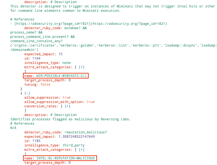
This also illustrates how each event can exist on a one-to-many relationship with detectors. In the screenshot above, the engine_observations (detector) section has two sections for two detectors: WIN-POSSIBLE_MIMIKATZ_CLI and INTEL-RL-REPUTATION-MALICIOUS.

This is great for the analyst to determine potentially malicious behavior, but it’s not as good for individual detector metrics or some of the statistical functionality of Splunk. We currently use mvzip and mvexpand in order to get a searchable detector and corresponding id per event. While this will cause duplicate events, it’s okay for our purposes.

The image below shows the results when stats are used within Splunk. Using “expand” yields the following, which now counts the single event as two.

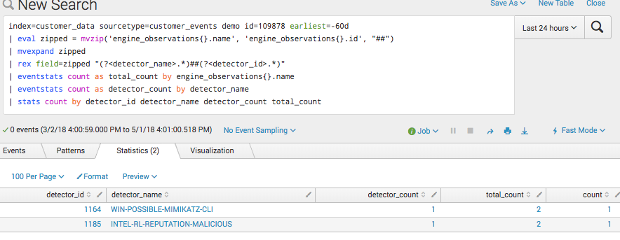Our base query ends up looking like this. Essentially, we’re taking all of the events that are not handled by automation and breaking them out by detector name. The numeric id we use to identify each unique detector.

index=customer_data sourcetype=customer_events analyst!=*bot*
| fields engine_observations{}.name engine_observations{}.id claimed_at terminal_at terminal_stage associated_detections{}.headline
| eval zipped = mvzip('engine_observations{}.name', 'engine_observations{}.id', "##")
| mvexpand zipped
| rex field=zipped "(?.*)##(?.*)"

Step 2: Calculate Conversion Rate

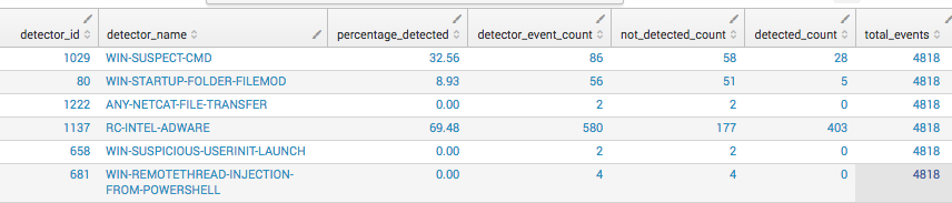
We need two things in order to get the conversion rates for each detector: a count of detected events and the total events by detector.

This code gets added to the base query:

| eventstats count as "total_events"
| eventstats count as "detector_event_count" by detector_name
| eventstats count(eval(terminal_stage="hidden" OR terminal_stage="hidden_not_suppressed")) as not_detected_count,count(eval(terminal_stage="detected")) as detected_count by detector_name
| eval percentage_detected=round(detected_count/detector_event_count*100,2) | table detector_id detector_name percentage_detected detector_event_count not_detected_count detected_count total_events | dedup detector_name

By building the query in sections, it’s easier to cross check it against raw data to see if the results are correct. We don’t technically need the “not detected” count for conversion, but it can be a handy metric. This also gives us the total events per detector and total events for the time period, which we’ll use later.

Step 3: Calculate Time Claimed

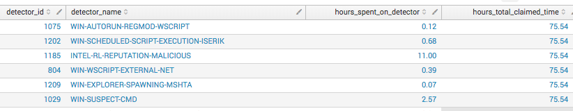
The next metric is “time claimed per detector.” This metric is helpful in determining which detectors take more human analyst time to look into than others. We track the timestamp of when an analyst ‘claims’ an event to when it’s ‘terminal,’ which is the time it takes before an analyst takes an action.

This calculation can be high because of repeat events from the base query, but overall accuracy is good enough for our purposes. We take the difference between when an event was claimed and when it was terminal, then sum it to give us the time spent per event. The total sum gives us ‘actual’ hours spent across all events. This number is converted to hours because it’s easier for us to quickly make sense of.

The next part of the query looks like this:

| eval work_started=strptime(claimed_at, "%Y-%m-%dT%H:%M:%S.%3NZ")
| eval work_ended=strptime(terminal_at, "%Y-%m-%dT%H:%M:%S.%3NZ")
| eval time_worked=(work_ended-work_started)
| eventstats sum(time_worked) as total_all_events_claimed_time
| eventstats sum(time_worked) as total_detector_worktime by detector_name
| eval hours_spent_on_detector=round(total_detector_worktime/3600,2)
| eval hours_total_claimed_time=round(total_all_events_claimed_time/3600,2)
| table detector_id detector_name hours_spent_on_detector hours_total_claimed_time | dedup detector_id

Which results in the return of this data:

Step 4: Determine Acceptable Thresholds

So far we’ve determined what we’re going to measure and how to break out the numbers by detector. Now we need to determine what acceptable thresholds are. The first iteration involved just doing some calculations based on estimated levels of effort.

Here’s an example to illustrate: Let’s assume there are 10 full-time analysts investigating events 100% of the time (which is unrealistic but helpful for our example). This yields 400 hours of human time a week. On average, we can estimate that an analyst can get through about 30 events an hour. Multiply that by 400 hours, and this means we want to avoid generating more than 12,000 analyst-handled events a week.

A lot of math has already gone into figuring out human time, both how much time we actually spend on events and how many events we can handle for staffing reasons. For our current team, we’re going to factor 254 hours of dedicated event investigation per week, which more realistically accounts for non-event investigation tasks that we encounter on a weekly basis. The event rate we tend to get through is actually much higher; let’s assume an average of about 23,500 a week.

Step 5: Putting It All Together

Recently we experimented with a scaled weighted average. Our first pass at that actually seems to be working fairly well at validating our confirmation bias of which detectors are the “worst.”

detector_score =
(detector_event_count/average_events*100) + (hours_on_detector/available_analyst_hours*100*weighting) -
(conversion_score * weighting)

We decided to weigh time pretty high at 0.75, because if 1,000 events take 2 seconds a piece, that’s approximately 33 minutes of human time and is not all that impactful. Conversely, if we only get a handful of events, say 15, but take 10 minutes to analyze, that’s about 2.5 hours of human analyst time.

Conversion is weighted at 0.25 and subtracted from the total, because the higher the conversion, the more accurate we presume the detector to be. The event rate is not weighed at all. Because conversion is weighted so high, there are often negative scores. The more negative the score, the better the detector actually is. While this may not be statistically perfect or mathematically accurate, within this iteration it’s working for our purposes, and we aim to improve it over time.

Here’s what this looks like implemented over 7 days:

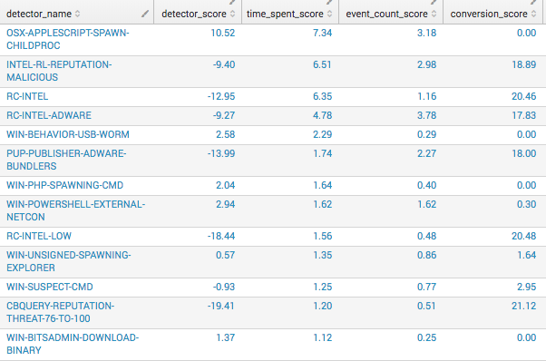When we combine everything above, we get the massive query seen below. This gives us all the numbers we need and then calculates the score in preparation for running a weekly report. If performance were an issue, this would probably need to be reworked, but this search is running about once a week, so it’s okay that it can take some time to churn through.

index=customer_data sourcetype=customer_events analyst!=*bot* earliest=-7d@d latest=@d
| fields engine_observations{}.name engine_observations{}.id claimed_at terminal_at terminal_stage associated_detections{}.headline
| eval zipped = mvzip('engine_observations{}.name', 'engine_observations{}.id', "##")
| mvexpand zipped
| rex field=zipped "(?.*)##(?.*)"
| eval average_weekly_event_rate=23500*4
| eval total_analyst_available_hours=254*4
| strcat "https://master.my.redcanary.co/detectors/" + detector_id detector_link
| eventstats count as "total_events"
| eventstats count as "detector_event_count" by detector_name
| eventstats count(eval(terminal_stage="hidden" OR terminal_stage="hidden_not_suppressed")) as not_detected_count,count(eval(terminal_stage="detected")) as detected_count by detector_name
| eval percentage_detected=round(detected_count/detector_event_count*100,2)
| eval work_started=strptime(claimed_at, "%Y-%m-%dT%H:%M:%S.%3NZ")
| eval work_ended=strptime(terminal_at, "%Y-%m-%dT%H:%M:%S.%3NZ")
| eval time_worked=(work_ended-work_started)
| eventstats sum(time_worked) as total_all_events_claimed_time
| eventstats sum(time_worked) as total_detector_worktime by detector_name
| eval hours_spent_on_detector=round(total_detector_worktime/3600,2)
| eval hours_total_claimed_time=round(total_all_events_claimed_time/3600,2)
| eval conversion_score=round(percentage_detected*0.25,2)
| eval event_count_score=round((detector_event_count/average_weekly_event_rate)*100,2)
| eval time_spent_score=round((hours_spent_on_detector/total_analyst_available_hours)*100*0.75,2)
| eval detector_score=round((time_spent_score+event_count_score)-conversion_score,2)
| bin _time span=1d
| eventstats count AS hits BY detector_name,_time
| eventstats max(hits) as top_day by detector_name
| eval high_day_percentage=round(top_day/detector_event_count*100,2),mean_a_day=round(mean_a_day,0)
| table detector_name detector_score detector_link time_spent_score event_count_score conversion_score hours_spent_on_detector detector_event_count top_day high_day_percentage percentage_detected hours_total_claimed_time total_events
| dedup detector_name | sort - detector_score

Step 6: Track Results

We scheduled the query to run once a week and e-mail the results to us. We go through this list manually because there are other factors that influence this. We also use GitHub to create and track an issue for each detector that is scoring high. The detector will be evaluated to determine:

• Can we make any improvements?
• Is it too noisy to be useful?
• Is it covered elsewhere?
• Do we need to leave it alone?

Currently we evaluate the last 28 days, but it’s very easy to adjust the timeframe.

Applying Detector Scores to Evaluate Performance

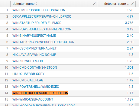
All of the previous work laid the groundwork to score each detector so they could be ranked in a repeatable way to evaluate detector performance on a weekly basis. The higher a detector’s score, the worse it’s performing.

For example, in March, WIN-SCHEDULED-SCRIPT-EXECUTION – 501, showed as 14th in detector rank, out of 328 we saw in that period.

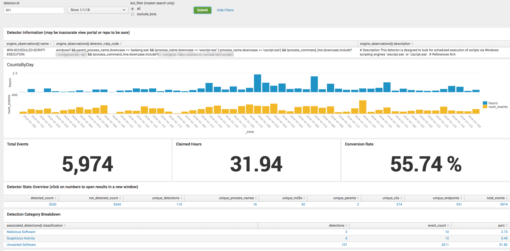
By putting all the pertinent information into a dashboard, we can simply input a detector id to answer common questions on detector performance.

The screenshot below shows an overview of the WIN-SCHEDULED-SCRIPT-EXECUTION detector since January of this year. You can see via the timechart of hours worked and number of events that it’s a fairly consistent detector because it wasn’t noisy one week, then quiet after that. These numbers include all events that are handled by automation.

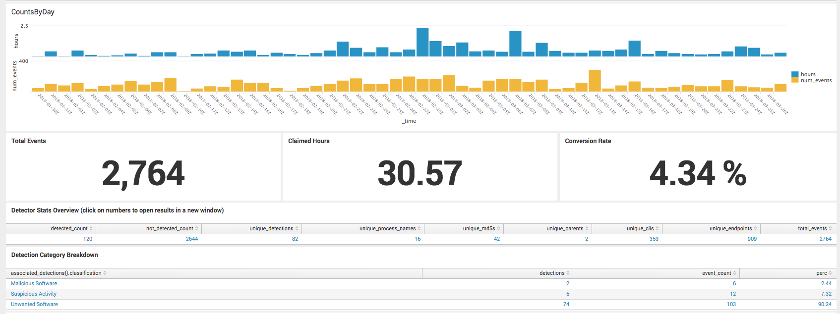
If we look at the numbers without automation, we can see that it clearly plays a large role in this detector. It is also the reason why we want to improve it. Looking at the number of total events, 2,764 out of 5,974 is still a relatively large number of events. You can see the claimed time has stayed right around 30 hours, but now only only 4% of the human-handled events convert into detections.

Let the Tuning Begin!

The first step in detector tuning should be to look at its code because sometimes logic errors can inadvertently get overlooked when we initially push the detector live, but more importantly, it shows exactly what the detector is looking for. In the following case, the detector is looking for a windows OS, with taskeng.exe executing either wscript.exe or cscript.exe.

windows? && parent_process_name.downcase == 'taskeng.exe' && (process_name.downcase == 'wscript.exe' || process_name.downcase == 'cscript.exe')

One of the things we rely on to reduce and filter the events we see from a given detector is suppression. Suppression means that we make a rule saying, “If a process meets certain criteria, don’t create an event and don’t show it to the analyst.” However, our options for suppression are generally limited to process MD5, parent process MD5, and command line. Notice this detector specifies both a parent and a process name specifically, so the only suppression option here is going to be command line. This can work well if there are a lot of repeat command lines, but less well if the command lines vary. Think of dates or some other kind of incrementally changing output filename.

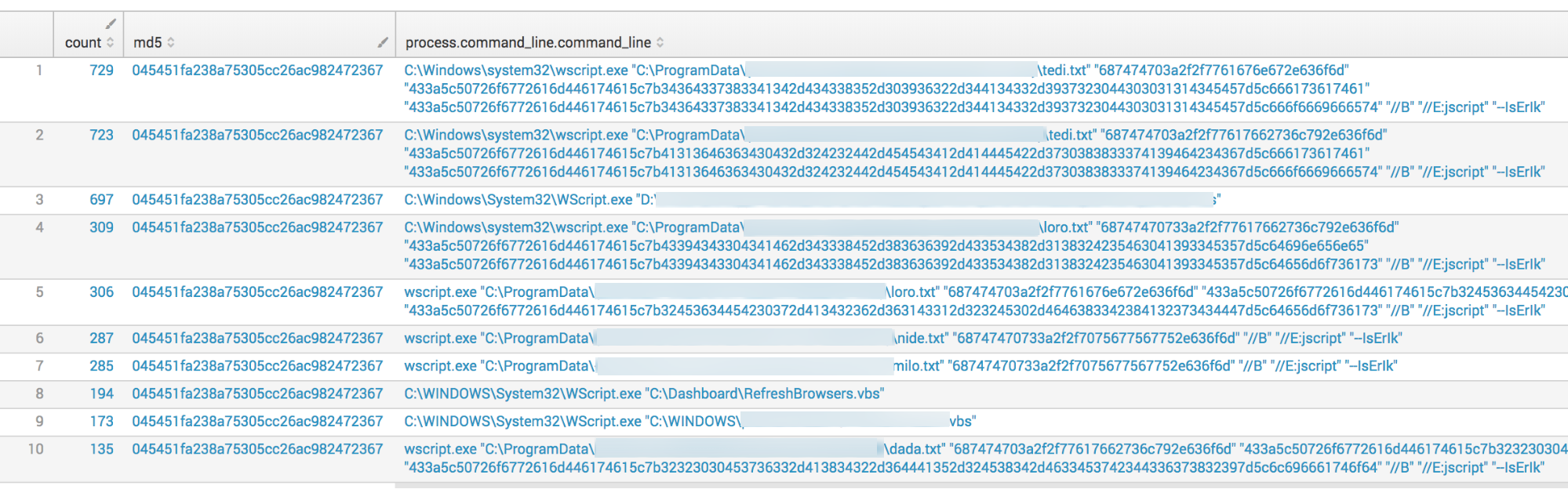
When we take a closer look at WIN-SCHEDULED-SCRIPT-EXECUTION – 501, there have only been 378 unique command lines out of almost 6,000 events, which means we’re seeing a lot of the same events. This makes sense, because a good portion of them are being handled without humans. The screenshot below shows the top command lines (CLIs) given and already a fairly distinguishable pattern can be seen in the top 10 results.

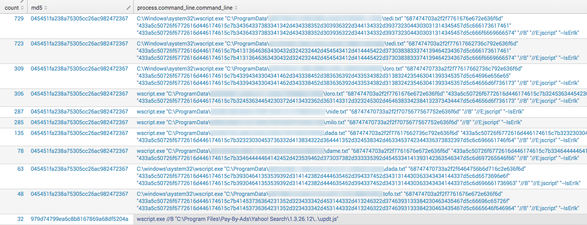
The next logical step is to see if these similar CLIs fall mostly in the detected or not-detected category for the detector. It turns out that of those unique 378 CLI’s, not-detected events make up 336 of them. This helps explain why the automation is handling so many events, because about half of the events are comprised of the same MD5 hash and CLI. The detected events are predictable; the non-detected events are more scattered and unique. This indicates that suppression is probably not having a widespread effect on the remaining events we see.

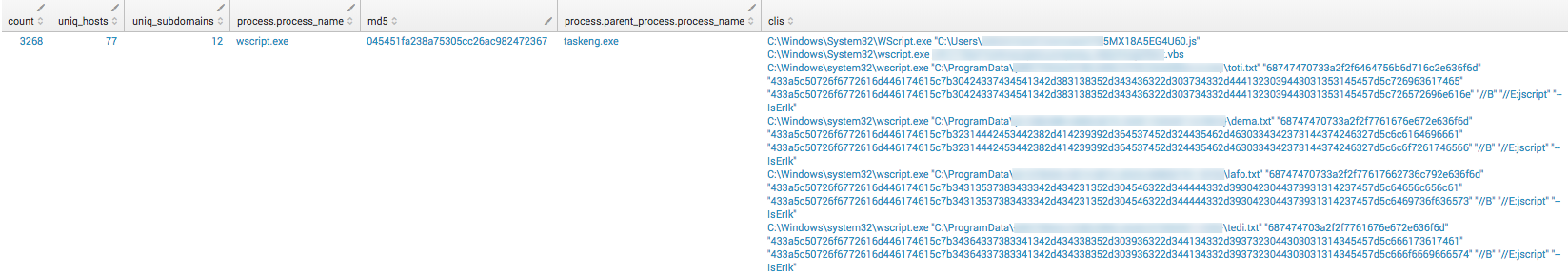
Sometimes a detected event type will be very noisy on one host, or one subdomain, but in this case it’s fairly widespread on 77 hosts across over 10 subdomains. The right column is simply listing out the unique CLIs seen with the hash/process_name combination; again, we see a fairly distinct pattern.

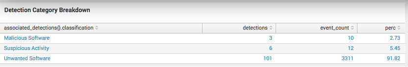
The next step is to drill into the actual detection composition for this detector. Right away we notice that this detector has almost exclusively been detected as part of Unwanted Software (Adware, Riskware, Peer-2-Peer) with 91% of detections, and all but 22 out of 3,000+ detected events.

At this point it makes sense to look at the Unwanted detections and the Malicious/Suspicious detections separately to see if there’s anything about these that differentiates them from the 2.6k events that were not part of a published detection.

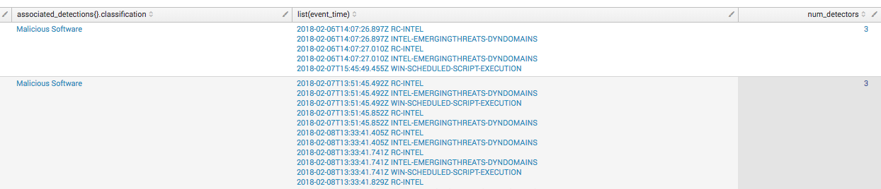
Clicking on the detection category opens a drilldown with the actual detections that contained events from this detector. In the image below, suspicious detections named this detector as the primary method of detection.

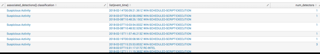While malicious detections were a bit more varied in coverage, having several types of detectors that were triggered. In both cases it was not enough additional coverage to make this detector completely redundant. This means that we don’t want to just turn it off.

Reviewing the details of a sample set of the malicious and suspicious detection events associated with the detector yielded the following CLIs:

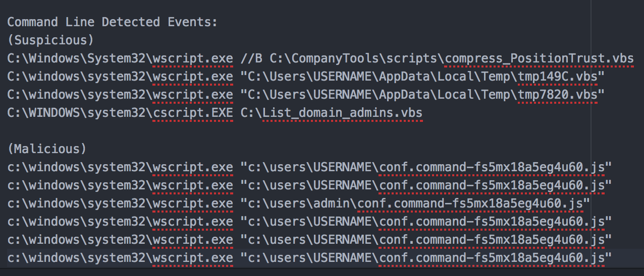In almost all of these cases the script in question is located in the Users directory, and the two that are not could likely be better detected in a different fashion. As a result of reviewing this data, a new detector idea is to add a quasi “path” check to make sure that the term users appears somewhere in the command line. We then add the term to the Splunk query to see how it would impact detection.

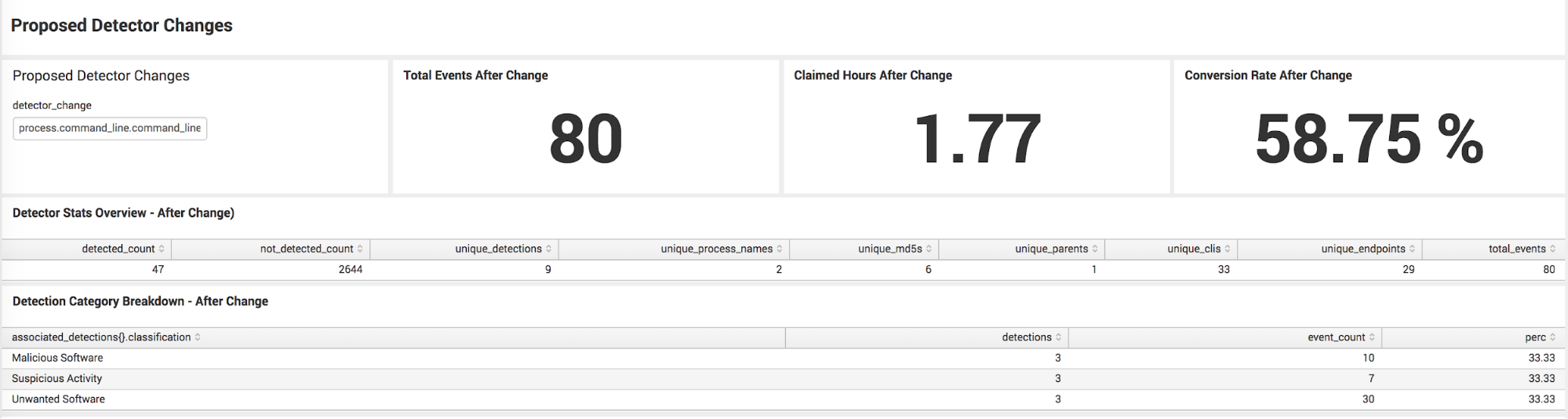
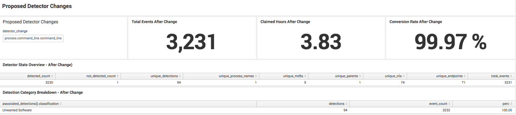
windows? && parent_process_name.downcase == 'taskeng.exe' && (process_name.downcase == 'wscript.exe' || process_name.downcase == 'cscript.exe') && process_command_line_downcased.include?('users')

Plugging the proposed change “process.command_line.command_line=*users*”
into the Splunk dashboard shows that if we add this criteria to our detector, the event count goes down to 80, whereas before it was over 2k, and the conversion rate goes up to 58%. A manual review shows we’re not missing any critical detected events with this change.

That’s a huge improvement, but what about the unwanted detections? It turns out that these are also fairly specific in the path that is used, and actually have a specific keyword as well. Adding a check for the path “programdata” in the command line, as well as the keyword “-iserik” – will give us a very specific unwanted detector to handle the rest of the events. We want to use two detectors instead of lumping this into one because it gives us more options for automation.

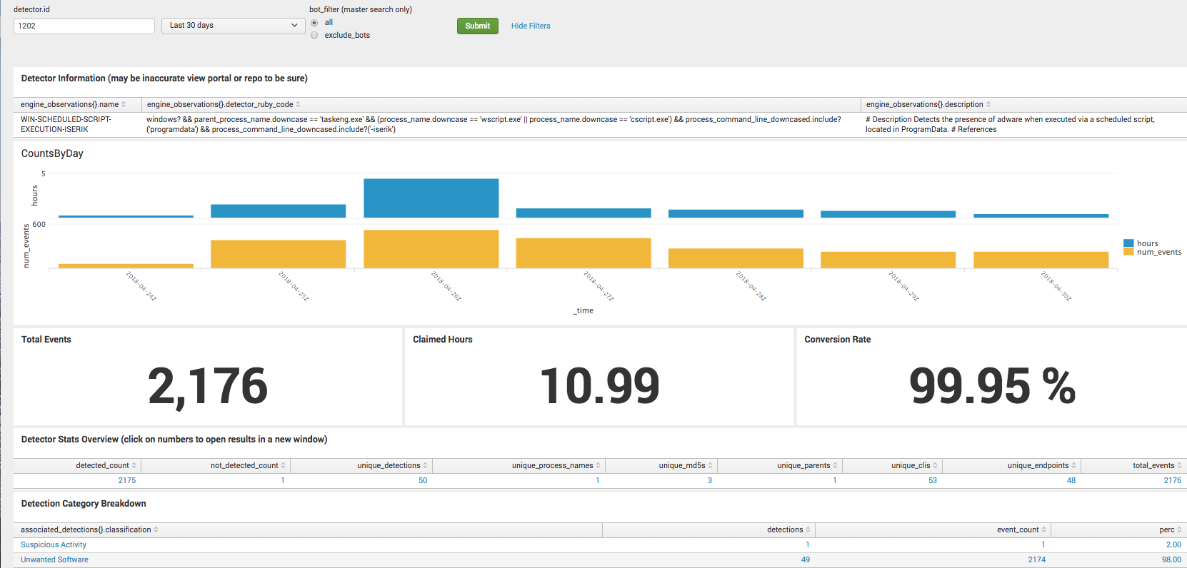
windows? && parent_process_name.downcase == 'taskeng.exe' && (process_name.downcase == 'wscript.exe' || process_name.downcase == 'cscript.exe') && process_command_line_downcased.include?('programdata') && process_command_line_downcased.include?('-iserik')

Adding the terms shows a conversion rate of 99.9%

We can now deactivate the original detector, and instead will put into place two separate detectors. Yes, there may be a few cases where we want to look for a different path, but we had a fairly large dataset that spans over 4 months—so we can be reasonably sure that breaking these detectors out will not significantly reduce coverage—and the potential benefit is cutting down a large swath of noise for the analyst team to review.

Impacts from Detector Tuning

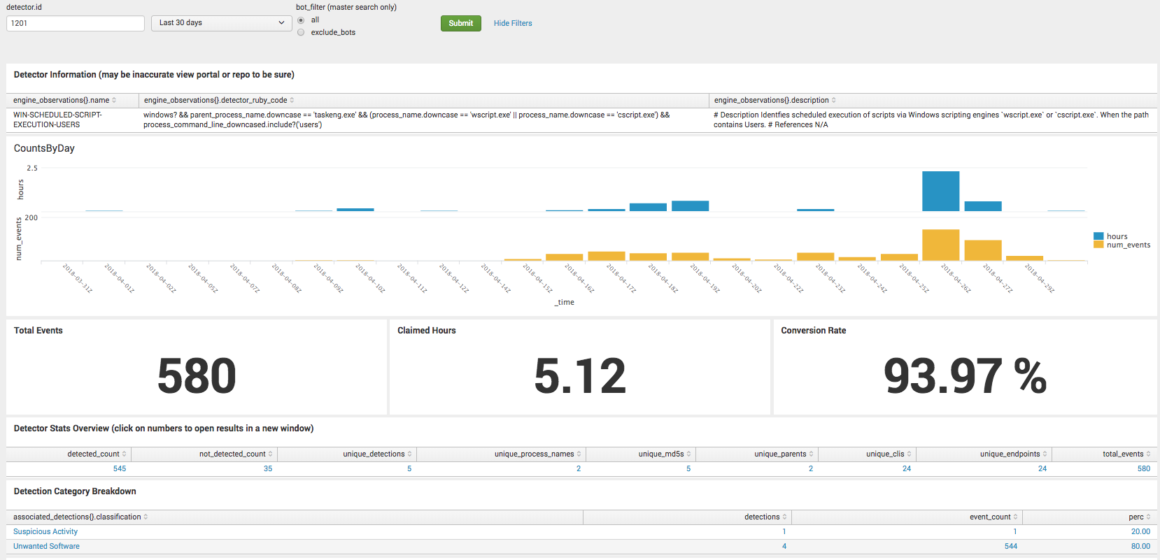
Since this was recently implemented, we have the actual results for these two detectors. The changes resulted in increasing the human handled conversion rate from 4% to 93% and the bot-handled conversion rate from 55% to 99%. Not all results are this drastic, but it’s a fairly good example of one where a bit of research yielded a big change in conversion rate. Here are the screenshots for the conversion rates for the respective detectors.

1201 – WIN-SCHEDULE-SCRIPT-EXECUTION-USERS – Last 30 Days

1202 – WIN-SCHEDULED-SCRIPT-EXECUTION-ISERIK – Last 30 Days

Continuous Improvement

Most of our team’s work thus far has been pulling together the initial statistics. Going forward, we’ll want to look at things like improved detector conversion rates, less time spent, and event count decreases. We can use the month-to-month score to see if a detector is improving or getting worse. Some remaining challenges include accounting for spikes, bugs, and other issues that can cause outliers that are not a true indication of performance.

We hope this behind-the-scenes look at Red Canary’s approach to tuning and detection engineering has been helpful. Every analyst out there has most likely experienced the fatigue that comes from sifting through piles of alerts. Applying engineering concepts to develop and tune detectors enables our team to filter out noise so we can focus on what matters: finding threats.

Take a deeper dive by watching an on-demand webinar with CEO Brian Beyer: Opening the Floodgates: How to Analyze 30+ TB of Endpoint Data Without Drowning Your Security Team